


|
|
|
|
|
|
|
|
|
|
The present page explains some topics, terminology and techniques that have been applied in Voynich MS text analyses. Some of these terms are used also outside the text analysis section. The representation of the Voynich MS script was explained on the analysis home page.
The first thing any analyst of the Voynich MS is likely to do is to count and make frequency tables of single characters, pairs, etc. and to do the same with the (apparent) words. When doing this, it appears immediately that some statistical properties are quite different for different parts of the MS, and appear to be strongly page-dependent. This was already noticed by Th. Petersen in the 1930's and indicated in his hand copy of the MS (1).
It was first analysed in some more detail by Prescott Currier in the 1970's. Currier indicated that the Voynich MS appears to have been written in two languages, which he called A and B. He was careful to point out that these are not necessarily different languages, but could be dialects, subject matter or different encryption, in case the MS has been written in a code or cipher. Since Currier also detected two handwriting styles (which he called 1 and 2) and found a perfect correlation: all pages in language A were in hand 1 and language B was in hand 2, he concluded that the MS had to be the work of at least two people. In fact he suggested further hands which he called 3, 4, X and Y, but while the languages A and B and hands 1 and 2 are easy to recognise, the other hands have not become as generally accepted.
Currier presented his findings in detail during a symposium about the Voynich MS which was held on 30 November 1976 and led by Mary D'Imperio. Currier's paper has been converted into electronic form. This HTML version only has the main text. The full paper with all the long tables is available also in separate files in PostScript format at a >>page prepared by J. Reeds and mirrored by J.Stolfi or, converted to PDF, via this link.
The Herbal section appears to be a mixture of A-language and B-language pages, and the distribution of these pages was strictly according to the bifolio, i.e. entire bifolia are always written in one language. He also saw two different handwriting styles which were fully correlated with the type of language. This has already been shown in a previous page.
The main properties which Currier gave for his two languages are:
The above shows that the Currier language is evident from criteria based on single characters, character groups and whole words.
After some initial experimentation around the year 2000, which has been reported here and here, in April 2024 I made a first iteration of a new classification of languages in the Voynich MS, into three "RZ" languages (A, B and C), and a few 'dialects' of these languages.
In general terms, RZ language A coincides with Currier language A. RZ language C has properties that are in between Currier languages A and B, and it is found in most of the astronomical and cosmological pages that Currier did not classify. Some of the pages Currier classified as B language coincide more with RZ language C than with RZ language B.
Details of this new classification may be found here. Both the Currier language and RZ language identifications have been included in the summary page descriptions that are linked through this page.
The entropy of the language of the Voynich MS was first studied by Bennett (1976) (2), and when his estimates turned up rather anomalous values for the Voynich MS text, compared with most European languages (old and new), this became an important topic for subsequent investigations. The meaning of entropy is therefore introduced in some detail here. Note that this is not a very formal mathematical introduction, but mainly one aiming at allowing the reader to understand the various analyses that use it. Bennett refers to Shannon's important paper on "The Mathematical Theory of Communication", and a useful summary for the interested reader may be found >>here.
Entropy is a quantity that could be interpreted as amount of 'chaos' or unpredictability, in the sense that lower values of entropy are equivalent with higher amounts of order or predictability. This can be applied to the analysis of written text as follows. If a string of characters has full predictability, it carries no information. Once one knows the first character, one can predict all subsequent ones: one knows everything. The entropy of a piece of text is therefore also a measure of the amount of information it carries. The entropy values used in the study of the Voynich MS text are usually expressed in bits (of information).
This is best elaborated using a simple example.
Imagine someone were to create a string of numbers using a die. He would roll the die, write down the top face number, and repeat this process as long as he wanted to. The number that appears each time (at each event) is a piece of information. The amount of information is inversely proportional to the probability of the event, and is usually expressed in 'bits', by taking the base-2 logarithm. If the die is a perfect 6-face die, then the probability (p) of throwing a '1' (or any other number) is 1/6. The number of bits of information (b) obtained at this event is the base-2 logarithm of 1/p, or:
![]()
On average, the number of bits of information obtained at the appearance of each number (which is the entropy, denoted here by a capital Greek Eta: Η) is the weighted average of all possible outcomes:
![]()
In our example of a string of text (whether digits or characters) generated by throwing a perfect 6-face die, the entropy on a single-character basis is:
![]()
Had the die not been perfect, but weighted, the six probabilities would not all have been equal to 1/6, and the resulting entropy value would have been lower than the above value. (A mathematical proof of this is straightforward but outside the scope of this page). The die is a bit more predictable (has a tendency towards the most probable number) and the entropy is lower.
Had the die not had 6 sides but any number N, the maximum entropy (in case all probabilities are equal) would have equalled
![]()
The main point resulting from the above is that the entropy is a value that can be computed for something which can assume a number of values, and the sum of the probabilities for each of the values is one. One could use the index i to denote each of the values, and p(i) the probability that the 'thing' has value i. The formula for the entropy of this is:
![]()
For a piece of text, the single-character entropy can be computed using the probabilities of the occurrence of each of the characters of the alphabet. For a text written in an alphabet of 26 characters, this entropy will be less than 2log(26) or 4.700, knowing that not all 26 characters will appear equally frequently. Of course we don't know the real probability, but we can only estimate it by looking at the frequency of occurrance, and assuming that this is close to the probability. This will be reasonable for sufficiently large samples, but not in case a text is not sufficiently large to capture rare characters or combinations of characters properly.
It is therefore important to keep in mind that the single-character entropy computed in the above manner for any piece of text in any language will only be an approximation of the true or inherent single-character entropy of that language. Apart from the above-mentioned approximation, there is also the issue that the entropy will depend on the subject matter and the writing style of the author.
The most important point is, that the entropy does not depend on which character set or alphabet is used, but only on the probabilities or frequencies. This means, that the entropy of a text does not change if it is subject to a simple substitution encoding. This is the main reason why the entropy is of such interest for the Voynich MS. The entropy also does not change, by the way, in case the text is written backwards.
Entropy can also be computed for words rather than single characters. A text written in a vocabulary of 10,000 words will have a word entropy less than 2log(10000) or less than 13.288, depending on the distribution of the word frequencies. It can furthermore be computed for character pairs. Going back to the example of throwing the die, there are 36 possibilities for a pair of throws. The entropy for this (assuming a perfect die) is
![]()
It is evident that if the occurrence of the two consecutive events is independent, the 'pair' entropy equals twice the 'single event' entropy.
In natural language, however, the occurrence of a character in a text is not independent from the previous character. For example, in English the probability of encountering the character 'u' depends highly on whether the previous character was a 'q' (in which case the probability is essentially 1), another 'u' (in which case it would be very close to zero) or anything else. This introduces the concept of conditional entropy. It can be shown mathematically that the conditional single-character entropy (the entropy of the probability distribution of a single character, given that the preceding one is known) equals the difference between the character pair (=digraph) entropy and the single character entropy. This conditional character entropy is less than the 'normal' character entropy.
A word on terminology: single-character entropy is sometimes called first-order entropy. Character-pair entropy is sometimes called second-order entropy, while the conditional single-character entropy is also sometimes called second-order entropy. The values given for these quantities should remove any doubt about what is meant, since the conditional second-order entropy is always less than the single-character entropy, while the character pair entropy is always greater than the single-character entropy.
Zipf's law (strictly the first Zipf law) concerns the frequency of words in a piece of text. If one orders the words according to decreasing frequency, i.e. label the most frequent word as nr.1, the second most frequent word as nr.2, etc, and then make a plot of the frequency of this word according to this rank, the result should show a straight line with a slope of -1, if both scales are logarithmic.
This general statement requires some elaboration:
The straight line with slope -1 in a double-logarithmic scale means that the probability for the item ranked at nr. i equals:
![]()
where C is a constant depending on the number of items N, and it is defined by the fact that the sum of all probabilities has to equal 1. Thus, if a quantity can assume a well-defined number of values, and it strictly obeys Zipf's law, its entropy can be predicted exactly.
Following is a table which illustrates this. The first column gives the number of possible values. The second gives the maximum entropy, if all probabilities are equal. The third column gives the entropy if the quantity exactly obeys Zipf's law. For example, the value 26 represents the number of letters in the (Latin) alphabet. If they are all equally frequent (which they are not), the character entropy would equal 4.700. If they exactly followed Zipf's law (which is also not true, but certainly closer to the truth), the character entropy would equal 3.929. The table has been set up for reasonable values of alphabet size, number of digraphs and number of words in a text.
  Number     H(max)   H(Zipf)

    16       4.000     3.403
    17       4.087     3.470
    18       4.170     3.532
    19       4.248     3.591
    20       4.322     3.647
    21       4.392     3.700
    22       4.459     3.750
    23       4.524     3.798
    24       4.585     3.844
    25       4.644     3.887
    26       4.700     3.929
    27       4.755     3.969
    28       4.807     4.008
    29       4.858     4.045
    30       4.907     4.081
    31       4.954     4.116
    32       5.000     4.149
    33       5.044     4.181
    34       5.087     4.213
    35       5.129     4.243
    36       5.170     4.273
    37       5.209     4.301

   100       6.644     5.310
   200       7.644     5.986
   500       8.966     6.851
  1000       9.966     7.489
  2000      10.966     8.115
  5000      12.288     8.927
10,000      13.288     9.532
20,000      14.288    10.130
50,000      15.610    10.911
|
Hidden Markov Modelling (HMM) is a statistical technique that was developed in the 1960's, but only found significant application considerably later. Analysis of written text on a character basis is only one of its many applications, and for the purpose of Voynich MS text analysis we may skip a more general description of HMM, and concentrate specifically on this case. The following largely follows the introductory paper of Stamp (2018) (3). A more general and easy-to-follow introduction to Markov chains (normal and 'hidden') is provided here.
HMM analysis of a text assumes that a sequence of characters that we observe can be modelled by another hidden sequence. For ease of understanding we may call this hidden sequence a sequence of 'types' (4). The number of different types is always much smaller than the number of different characters. A typical case is the classification of characters into two types: vowels and consonants.
HMM analysis essentially consists of an analysis of two processes: there is one process that defines how one (hidden) type causes the next (hidden) type. In the case of vowels and consonants, this is the process that decides whether the character following a vowel or consonant will be a vowel or a consonant. Then there is a second process that says which particular vowel or consonant is actually observed. The following figure from Stamp (2018)
(see note 3)
should clarify this.
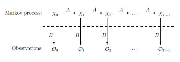
Process A describes the transition from one hidden type X to the next hidden type. Process B describes the transition from a hidden type X to an observed character O. Note that the analyst only sees the observations O, while the hidden types X (behind the dotted line) are not known, but can be estimated. The sequence of observations O is nothing more than the string of characters that make up the text.
Both processes A and B are stochastic, which means that they consist of a list of transition probabilities. In mathematical terms, both A and B are represented by a matrix.
HMM analysis now consists of computing the probabilities related to both processes, i.e. the numbers in the matrices A and B, based on an input text. The standard algorithm for doing this is called the Baum-Welch algorithm (5). The power of this analysis is that, indeed, it is capable of detecting vowels and consonants in strings of meaningful text in known languages, when it is being applied with two 'types'. It can also work with more than two types. An analysis of English based on two to five types was performed by Cave and Neuwirth (6).
Some HMM analyses of the Voynich MS text have been performed, and these are discussed in section 2: character statistics.
Many more tools have been applied since the MS has been available in machine-readable format (i.e. transliterated). Some of the more general ones are briefly described in the following. In addition to this, many people have introduced their own techniques which are described in their papers.
Cluster analysis is a method for classifying large sets of similar statistics into groups or clusters. It has been applied to the Voynich MS mostly to identify and classify properties 'per page' of the MS. This was triggered by Currier's identification of the differnt Currier languages (per page).
Typically, this method requires that for each page of the MS a quantitative attribute is found, which may consist of one number, but also a set of numbers. Next, it requires the definition of a 'distance' function which takes the attributes of any pair of pages and computes a distance value which should be low if the attributes are similar and high if they are dissimilar. Such quantitative values and their distances can be based on single characters, digraphs, words or any other property.
The complete set of distances between all pages then consists of a square matrix, where point (a,b) represents the distance between the properties of pages a and b. For usual and meaningful definitions of this distance, the value for (a,a) will be zero (since the properties are equal) and the value for (a,b) will be the same as for (b,a). The matrix will be symmetrical with respect to its main diagonal.
The final, and sometimes difficult task is then to decide, on the basis of the square matrix of distance values, which pages are similar (for example: written in the same language or on the same topic) and which are not. Then: into how many groups or 'clusters' the whole set of pages can be subdivided.
The Russian mathematician Boris V. Sukhotin devised several analysis techniques which were published in Russian. In the early 1990's they were translated by Jacques Guy. Best known is Sukhotin's algorithm to identfy vowels and consonants in a text (7), which has also been applied by Jacquest Guy. This is discussed in section 2: Character statistics. The other analysis techniques of Sulhotin are described in detail on a dedicated page.
This technique collects 'local' or 'regional' statistics of a text, analyses their variation over different ranges of the text, and detects patterns that may be typial for meaningful text. While applying these techniques, it is of interest to compare the original text properties with those of a scrambled version of the text (all words scrambled arbitrarily), and to analyse the differences. While long-range correlation analyses can present interesting results, their interpretation is not always easy. Some examples are given in section 5: Sentences, paragraphs, sections.
|
|
|
|
|
|
|
|
|
|