


|
|
|
|
|
Various cluster analyses of the pages of the Voynich MS have been performed, and each of these was able to show the clear difference between the Currier languages A and B, and the various flavours of Currier language B (1). These analyses were based either on the single character distribution using the Currier or FSG alphabets, or the distribution of Voynich words, which is almost independent of the chosen alphabet.
This page looks at the distribution of character pairs or bigrams over the pages of the Voynich MS, which could potentially give a very clear picture because:
To count bigrams, one should know what constitutes a single character and this is the first problem. The existing transliteration alphabets are probably all wrong in this respect (2).
The Eva transliteration alphabet is of analytical rather than synthetic nature, which means that certain Voynich characters which probably represent one character are written as a composite (such as 'ch' for and 'iin' for ). The Currier alphabet has the opposite problem. By translating the Voynich MS text to a more suitable alphabet, this problem may be reduced. In the following I will use a mixture of Eva and Currier, which I will call Cuva).
| Definition of the "Cuva" analysis alphabet |
It should be noted that this alphabet is only intended for use in statistical analyses, and is not suggested as a good transliteration alphabet. In particular the equation ⇒ , ⇒ (etc) may not be the best choice, but this was done in order to restrict the alphabet size to 26.
When all bigrams of the complete Voynich MS, transformed to Cuva, are counted, it turns out that 355 different bigrams exist. During this count, bigrams including Eva special characters were skipped. Furthermore, bigrams spanning word breaks were not counted and uncertain spaces were discarded (i.e. treated as 'no space'). There were 232 pages with some text, the ones without text being f101r2 and f116v. (The text seen on f101r2 was counted on f101r1, as the lines of text span both pages).
Next, the bigrams were counted on each page separately. The page length differs greatly. Short pages such as some Herbal-A pages had as few as 200 bigrams, but long pages such as in the stars section could have up to 3000 bigrams. One can arrange the 355 frequency values (the fractions) for each page in a vector of length 355, where the sum of all components of each vector equals one. Thus, 232 vectors arise, all contained in the quadrant where all components are positive. The vectors all point to a small region in 355-dimensional space.
It is more interesting to subtract from each of the vectors the one vector which represents the average bigram distribution for the entire MS. Now the vector for each page shows the way in which this particular page differs from the 'average MS page'.
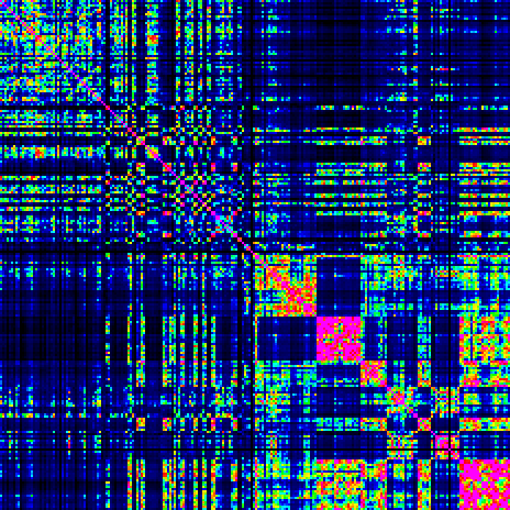
Pages with similar properties will be close to each other in this small hypercloud in 232-dimensional space, so their Euclidian distance will be small. This distance can be computed for each pair of pages, leading to 232**2 values which can be arranged in a square matrix (3).
The following plot shows a colour-coded 232 * 232 square matrix, where the page number increases from 1 to 232 from left to right and from top to bottom. The main diagonal (top left to bottom right) has values 0. The colour scale is such that large distances are dark blue going through light blue, cyan, green, yellow, orange, red to magenta for the smallest distances (4).
The first thing that appears is the checkerboard pattern showing that certain groups of pages have similar properties. It reflects the known alternation of pages in Herbal-A, Herbal-B, Biological, Pharmaceutical and Stars sections. To show these properties better, the same matrix can be plotted with the pages grouped per known section.
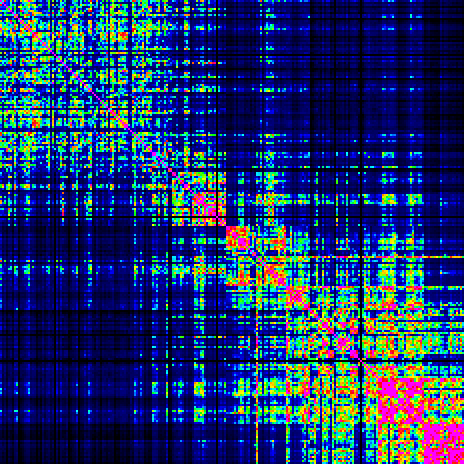
The pages have been reordered by the illustration countained in them (but also taking into account the split of the herbal section into Herbal A and Herbal B as defined by Currier):
Below is the same picture as before, but with the rows and columns now ordered as above.
It is possible to tentatively identify the following languages and dialects. The first character (capital) gives the language, and any other characters (lower case) a variation or dialect of this language.
Note that Bh and Bs may not be distinguishable, and the same
may be true for Bhb and Bsb.
Note also that there is some similarity between languages C, D and Ap.
To investigate further, it will be necessary to somehow quantify the smilarities and difference of all of the languages. As the hypercloud of points cannot be easily visualised in all its dimensions, various projections onto two-dimensional space may be tried out to discover the relation between all languages and dialects.
For certain bigrams, the relative frequency per page will vary significantly and for others this will be less the case. The frequency of such bigrams will tell a lot about the language or dialect used. The size of the hypercloud of points along this axis is larger than along other axes. It is of interest to find the vector in 355-dimensional space along which the size of the hypercloud is maximal. Then, the next largest direction perpendicular to it may be searched, etc, to find a small number of base vectors which form an orthonormal system, and which well describe the most important dimensions of the cloud.
The following procedure will not necessarily find this maximum, but it will find something near to the maximum.
Now, the coefficient along this base vector may be computed for each page vector. The contribution of this base vector may then be subtracted from each of the page vector, meaning that the hypercloud collapses to a space with dimension one less than before.
After this last step, the procedure may be repeated, and it will automatically find the next most important base vector, which will be perpendicular to the first. This whole procedure may be repeated several times.
The plot below shows the decomposition of all page vectors along the four most important directions. Base vectors 2 to 4 are plotted against base vector 1. Each small cross represents one page, and the colour of the cross depends on the illustration type as indicated (with the important exception that the herbal pages have been split into two, based on the already known differences in text statistics).
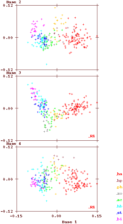
Clearly visible is that base vector 1 points along the direction from Biological to Herbal-A pages, as should have been expected. The rms variation of these coefficients is about 0.051, which is signficantly higher than the rms variation of any component of the page vectors (the maximum being 0.038). The most important conclusion from this plot is, that there is a clear correlation between the text and the illustration on each page in the MS. This is, because the location of any symbol depends only on the text, while the colour depends only on the illustration (with the important exception that the herbal pages have been split into two, based on the already known differences in text statistics). The different colours are clearly concentrated in different areas. This conclusion was later confirmed by the analyses of Montemurro and Zanette (2013) (5).
When Currier identified his languages A and B, he did this on the basis of the different statistics of the initial herbal pages in the MS, which are identified by the red ('A') and dark blue ('B') crosses. It is clear that these have distinct properties - the clouds do not overlap. He also checked the other pages, and noted more variations, but his criteria for distinguishing the languages did not allow him to see that the overall statistics demonstrate that there is a continuum, and the other (not herbal) pages actually 'bridge the gap'.
This does not demonstrate that the text is meaningful, or that the text variations are caused by different subject matter (as suggested in by Montemurro and Zanette). If that were the case, the difference between herbal A and herbal B should not exist. The cause of the (statistical) language variation is still unexplained.
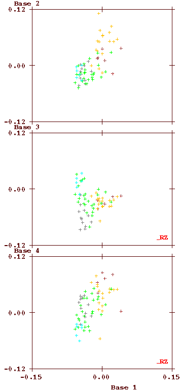
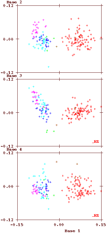
One feature which is not immediately obvious from the above figure is how much the language usage depends on whether the bifolio on which it is written has a standard size or has additional folds. To demonstrate this surprising feature, the plot is made again twice, below, on the left using only text on foldout bifolios and on the right only the standard-sized bifolios.
|
|
The 'bridging' between the two languages is located exclusively on the foldout pages. This is an important feature that equally still lacks an explanation, but which almost certainly must be related to the order in which the MS has been created.
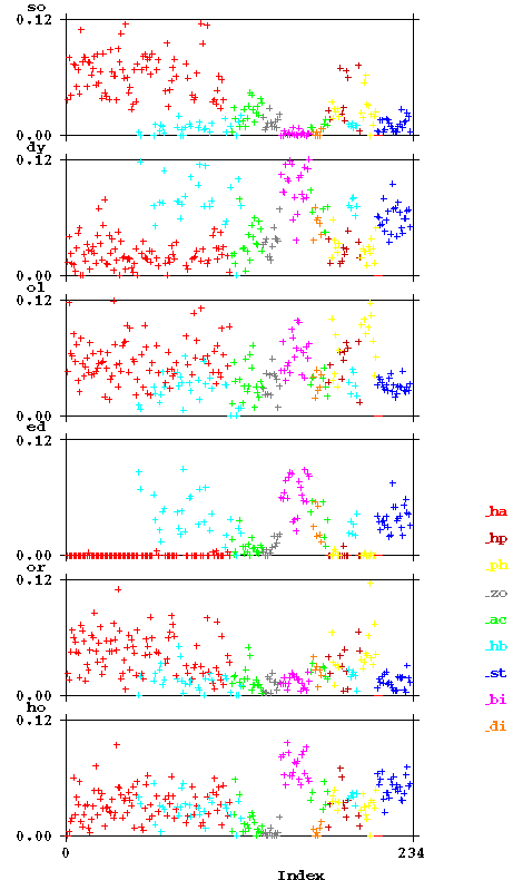
Further information may be obtained from the following plots, which show for some frequent bigrams (in Cuva though represented in lower case) which fraction they form on each of the pages. The first graph has the pages (on the X-scale) ordered as they appear in the Voynich MS. The second has them in the order described above.
|
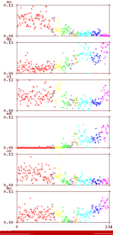
|
The colour again corresponds to the section of the MS as indicated by the two-character code introduced higher above (see between the two plots). The bigrams are indicated in Cuva (lower case). Some striking features, not reported by Currier in this form, are:
|
|
|
|
|