

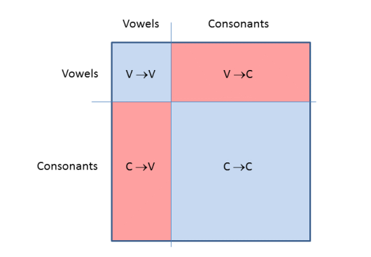
|
|
|
|
|
This page presents work in progress.
It is still subject to change.
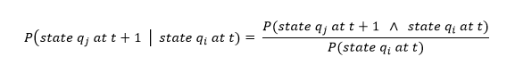
A brief introduction to Hidden Markov Modelling (HMM) was already provided here. Furthermore, an easy-to-follow general introduction to Markov chains (normal and 'hidden') is provided here. In the following, I will introduce an alternative approach to HMM processing. It is useful to have a fair understanding of how the standard HMM approach works. The terminology is first introduced in more detail.
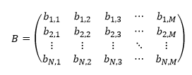
Central in HMM processing are the matrices A and B. Matrix A describes the transition probabilities from one hidden state to the next hidden state, while matrix B gives the probabilities that each state emits any particular character. The number of different states will be called N and the number of different characters in the text is M. The following largely follows Stamp (2018) (1), and probably most literature about HMM processing.
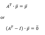
Matrix A is a square matrix. Each element describes the transition probability from one hidden state to the next hidden state. The first index, shown vertically, gives the present state and the second index, shown horizontally, the next state, as follows:
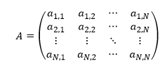
| (1) |
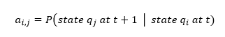
The meaning of each matrix element is: "the probability that the next state is j, given that the current state is i". In mathematical notation:
| (2) |
For each row in the matrix, the sum of the row elements is 1.
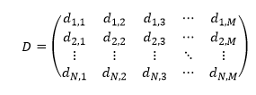
The B matrix is a rectangular matrix of size N x M. The first index, shown vertically, gives the state and the second index, shown horizontally, the emitted character, as follows:
| (3) |
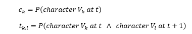
The meaning of each matrix element is: "the probability that the emitted character is k, given that the current state is j". In mathematical notation:
|
| (4) |
Again, for each row in the matrix, the sum of the row elements is 1. The notation bj,k is a more standard mathematical notation for the matrix elements than the notation: bj(k) that appears to be used in HMM publications.
For any N-state Markov process, the probability that each hidden state occurs is given by the vector of length N of average (hidden) state probabilities:
|
| (5) |
The average state probabilities do not play a significant role in the standard HMM approach, but they will in the following. In the standard HMM approach, a related quantity is the vector usually denoted as π0 , which gives the state probability distribution of the first character (2).
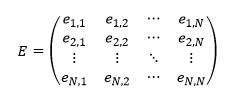
In the following, I will introduce alternatives for the A and B matrices. The E matrix is also a square matrix, with the same dimensions as A:
| (6) |
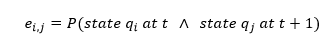
The meaning of each matrix element is: "the probability that the current state is i and the next state is j". In mathematical notation:
| (7) |
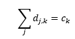
This means that for the E matrix the sum of all matrix elements is 1. Furthermore, we have for the sum of the row elements:
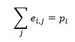
| (8) |
and the relation between the A and E matrix elements is given by:
|
| (9) |
This follows directly from the definition of the conditional probability:
| (10) |
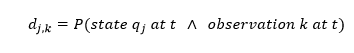
Similarly, we define matrix D as a rectangular matrix of size N x M, as follows:
| (11) |
The matrix elements are defined as: "the probability that the current state is j and the emitted character is k". In mathematical notation:
| (12) |
Also for the D matrix the sum of all matrix elements equals 1. Furthermore, the two following relations apply, in equivalence with the E matrix:
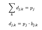
| (13a,b) |
Using the vector of average state probabilities, it is easy to convert back and forth between A, B and E, D. Also, if one has the E, D matrices, the average state probabilities can be computed trivially by summing the rows of either matrix. In the other direction this is different. It is not possible to compute the average state probabilities from the B matrix, but they can be derived from the A matrix by using the relation:
| (14a,b) |
This means that P is an Eigenvector with Eigenvalue 1 of the transpose of matrix A. Thus, P can be computed relatively easily with standard matrix operations.
The matrices introduced above will turn out to be helpful in analysing a piece of text. The HMM approach consists in optimising the A and B matrices (together with the π0 vector) such that they best replicate some property of the text that is being analysed. In the standard HMM analysis, the quantity that is optimised is the probability that this text could be generated by the pair of matrices. The detailed formulae for this process need not be included here, but the general approach is by starting with initial values for the two matrices and the vector, and iteratively improving them by processing the text.
The probability that the hidden Markov process reproduces the original text is defined as the probability that the first character is matched, times the probability that the second character is matched, times the probabilities that all next characters are matched. Since this will result in an extremely small number, the logarithm of this total probability is computed instead. The resulting value at the end of the process is usually not reported in papers, and appears meaningless, but if we divide it by the text length, we obtain the average probability that each character is matched. For the logarithm, I prefer to use the base-2 log. We will see later that this is a reasonably meaningful value to use.
Also the π0 vector obtained at the end of the process is considered to be of little interest, and is not usually reported. It will largely be ignored in the remainder of this page.
The algorithm that performs the optimisation of the matrices and vector is called the Baum-Welch algorithm, and it generally converges unless the initial conditions are chosen unfavourably. According to Stamp (2018) (see note 1), it may take of the order of 200 iterations. A disadvantage of the method is that it is quite unfriendly on computer memory as it requires storage of a matrix of size N x N for each character of the text (3).
It is usually necessary to pre-process the text to be analysed, by removing punctuation symbols and numbers, collapsing sequences of spaces into single spaces, and (depending on the language) converting upper and lower case to a single case.
When we perform an HMM analysis, we may take into account the character frequency distributions of the text being analysed. In the following we will call the vector C (of length M) the vector of single character probabilities, and the matrix T the matrix (of dimensions M x M) of character transition probabilities. The definitions of the vector and matrix elements are:
| (15a,b) |
For the T matrix, the first index is the left character of each pair, and the second index the right character. The probabilities can be estimated simply by counting occurrences in the text (frequencies). In the following, we will tacitly equate probability with frequency.
Representations of T matrices derived from a number of texts have been drawn in some pages at this web site, e.g. this page or this page. Further examples are included below on this page.
In order to have balanced statistics, it is a good idea to include an implicit space before the start of the text and one at the end of the text, and count the two as a single space. Effectively, it is as if the text starts again after the end, separated by a single space (the text is circularised). This has the advantage that there are as many character pairs as there are single characters, and the count of characters following a space is the same as the count of characters preceding a space.
However, the space character deserves further attention. In standard HMM analysis, this is simply considered one of the possible characters. An alternative would be to remove spaces completely from the text. A second alternative is to treat spaces as 'breaks' in the text. HMM analysis concentrates on the transitions between characters, so the choice has considerable impact. In the nominal case, transitions from a text character to a space, and from the space to another text character are treated as standard transitions. In the first alternative, there are no spaces, and transitions from the last character of each word to the first character of the next word are counted in the processing. In the second alternative, only transitions internal to words are considered.
Once an HMM using N states has been applied to a known text, we have obtained the best matching (according to some definition) A and B matrices. From these, we may also compute the P vector and the E and D matrices. We may now imagine that we let this Hidden Markov model run for a while, generating some text. In the following, we will call the output of this process the simulated text. We can now predict what will be the character and transition frequencies of this text, without actually generating this text.
Clearly, the simulated character frequency distribution should be equal to the actual character frequency distribution of the text. It follows from the definition of the D matrix that:
| (16) |
and therefore indeed the simulated character frequency distribution will be the same. For the simulated character pair (or character transition) frequency distribution we may write for each element of the simulated matrix S:
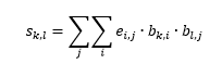
| (17) |
In matrix notation:
|
| (18) |
In the hypothetical (and not very interesting) case that we did an HMM analysis with only one state, then this single state will emit all characters with their known probability distribution. The resulting A and E matrices would collapse to the scalar value 1, and the B and D matrices would both equal the C vector (but transposed). In that case, the simulated transition frequencies become:
|
| (19) |
This represents a matrix where each element (each character pair frequency) is the product of the single character frequencies of the two characters.
As mentioned above, the standard HMM algorithm maximises the probability that the original source text could have been generated by the Hidden Markov process. We may now look for an alternative approach, in which the A and B matrices are chosen such that the resulting simulated character transition frequencies (as described above) are a best match for the actual transition frequencies of the plain text that is being analysed. The advantage of this is that it is not necessary to process a long text in several hundred iterations, but to work only (iteratively) with these frequency distributions. These frequency distributions can be computed by processing the text only once, and effectively the method becomes independent of the length of the text.
The above-mentioned relation between the B matrix and the C vector naturally gives rise to another useful rectangular matrix, which we may call R, as follows:
| (20) |
The meaning of each matrix element is: "the probability that the state is j, given that the emitted (current) character is k". In mathematical notation:
|
| (21) |
Now, for each column in the matrix (i.e. for each character), the sum of the column elements is 1. The relation between the R and D matrices is as follows:
|
| (22) |
All this means that the R matrix describes for each character, which state(s) is/are emitting it. Once we have this matrix, we can immediately compute the D matrix, from which follows the p vector, and from the two we can compute the B matrix.
But there is more. Knowing the R matrix and the transition frequencies of the text, we can also compute a matching E matrix. From the definition, each element of the E matrix gives the probability of the transition between two states. Since we have the probability distribution between any combination of characters (in T) and we have the probability distribution of each character over all states (in R) we can compute each element of E as follows:
| (23) |
or, in matrix notation:
|
| (24) |
From the E matrix we can then compute the A matrix. It can be shown easily by substitution of the relevant relations that the p vector computed from this E matrix is identical with the one obtained from the D matrix.
From a given (or assumed) R matrix we can therefore compute all needed quantities by using the known statistics of the text (given by C and T). We can then compute the simulated transition frequencies S, and compute a 'score' for this particular case by comparing it with the actual transition frequencies. This gives rise to an iterative procedure or algorithm which is described in the following.
Similar to the standard HMM implementation, this methods starts by setting up an initial or a priori matrix. In the standard case, both A and B are initialised with equal-probability values. In fact, and as described in literature, these values should be slightly offset from equal probability with some arbitrary offsets, in order for the process to start converging. In the present (alternative) method, only the R matrix needs to be initialised. This can also be done with near-equal probability values. The result of this is that the initial A matrix has near-equal probability values, while the initial B matrix already reflects the known single character distribution of the text. This is a clear advantage, and this is something that could also be used in the standard method.
As soon as we have an initial R matrix, but also whenever we have an updated R matrix, the following steps are executed:
For the score, the difference may be computed as the Bhattacharyya distance, a method also used in Hauer and Kondrak (2016) (4). In the present approach, this score has to be minimised using the iterative procedure.
Next, one needs to decided whether another iteration is needed. Different criteria for this may be used. If another iteration is needed, then the R matrix is adjusted in some way, and the process is repeated from the top of the numbered list above.
The difficult part of the process is to find a successful method for adjusting the R matrix. This is critical in order to achieve that the optimal solution is found. Intuitively, it seems that it should be possible to find a derivative of the Baum-Welch algorithm that works for this case, but this has not yet been achieved.
In an experimental implementation of this alternative method, a genetic algorithm has been implemented. This has some disadvantages: it is very inefficient, as it will typically require an excessive number of score evaluations. It is also not absolutely certain to be able to reach the true optimum. This will also be addressed further at a later stage.
Initial experimentation has shown that treating word spaces as 'just another character' is not entirely satisfactory. Clearly, spaces behave differently from normal characters, and spaces will never be followed by another space by convention (as described above under text pre-processing). This can be solved quite elegantly with the present method, because it is easy to define one additional state, which is forced to emit only the space character. At the same time, none of the other states are ever allowed to emit a space character. We will call this the space-only state in the following.
This has been implemented in the above-mentioned experimental implementation as an option. The average state probability of the space-only state is known from the beginning, and can be fixed. The entries in the R matrix for this character and this state are also known from the beginning and fixed. The calculation overhead for adding this special state is minimal, and experience shows that resulting scores with this approach are better.
The above-mentioned algorithm has been implemented, and, in addition, the standard Baum-Welch has been implemented as a separate application.
Whereas the Baum-Welch algorithm reads the text, the alternative method does not read the text, but only the character and bigram frequencies C and T. In the implementation used here, also the Baum-Welch algorithm reads these two quantities, where C is used to create a better initial B matrix, and T is used to compute the same score after each iteration as in the alternative algorithm, as follows:
This means that this method has two statistics to evaluate its success: the average logarithm of the character match probability ("log(prob)" in the following), which is the quantity being maximised by the algorithm, and the matrix difference, which should be observed to decrease, in case the process is successful. In the alternative method, 'log(prob)' is not available, but only the matrix difference, which is the quantity being minimised by the algorithm.
Both tools create an identically formatted matrix dump file. These matrix files can also be used as input by both methods, to provide the initial state for the iterative process (5). This means that it is possible to continue a process in case it is deemed that it may not yet have converged completely. However, it is also possible to continue an HMM process by switching the algorithm. Since the two algorithms are quite different, they are not expected to converge to the same optimum, so this is an especially interesting method to study the results. Finally, just doing one iteration of Baum-Welch after completing the alternative method allows to computed the 'log(prob)' score for this solution, which is not directly available in the alternative method.
With respect to the 'log(prob)' score, we can also estimate an a priori value of this quantity, which may help to evaluate the success of an HMM process. The C vector provides the individual character probabilities for the given text. If we generate an arbitrary text just based on these probabilities, we obtain an average match probability per character which is the sum of the squares of these probabilities.
One fundamental difference between the two methods needs to be highlighted. Whereas the Baum-Welch algorithm optimises two matrices, the alternative method only optimises one matrix, from which these two can be derived. This means that there is a relationship between these two matrices that does not necessarily exist in the case of the Baum-Welch algorithm (6). After every iteration of the Baum-Welch algorithm it is possible to not only evaluate the score as the matrix difference based on the A and B matrices (using the steps described above), but also to compute R and then the E matrix derived from R. This E matrix is observed to be indeed not equivalent with the algorithm's 'own' A matrix, and the corresponding 'secondary' score is always a bit worse than the algorithm's own score.
A genetic algorithm has been implemented in the alternative method. This is because for higher states it is not possible to try all possible permutations, and there are likely to be multiple local optima which will not be found by traditional hill-climbing methods. Of course, there is no guarantee that this genetic algorithm will find the correct optimum solution, so the implementation is still very experimental. It may be summarised as follows:
A final comment concerns the space-only state that can be used in the alternative method, as has been described above. For comparison purposes, it is of interest to do the same in the Baum-Welch algorithm. This has not yet been fully investigated, but it has been observed that it is possible to force such a space-only state, by initialising the two matrices and the vector accordingly (7). As it turns out, letting the process run will preserve the space-only state, and no other state will emit the space character. While this appears to work, this comes with the complete overhead, in terms of memory and CPU time, of using an additional state. This should not be necessary, and a more efficient method still needs to be designed. Furthermore, we shall see below that this method is not (yet) funtioning properly in all cases, and requires further analysis.
Earlier experimentation with the alternative HMM approach is the topic is described on this page (now outdated). The updated method is described in the following, using in parallel the Baum-Welch algorithm, to analyse a specific case in full detail. The implementation of both methods has been verified using a test case (8). Apart from that, the use of a space-only state with the Baum-Welch algorithm is still experimental.
In the following, the text used to illustrate the process is the Latin text of a so-called alchemical herbal from the beginning of the 15th century (9). After cleaning up (removing punctuation, consecutive whitespace and converting all to lower case) this text consists of 38,496 characters, including the additional space after the end of the text. The character pair frequencies are shown in square matrices with the first character of each pair on the vertical scale and the second character on the horizontal scale. The frequencies are converted to a colour as shown below the plot. In Figure 1 the characters are sorted alphabetically. The space character is included as the first character in the plots. In the left hand plot, the figure shows the character pair frequency as measured from the text (by simple counting).
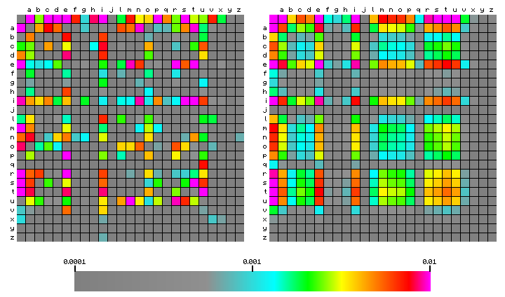
Figure 1: character pair frequency distribution for the alchemical herbal
Latin text, sorted alphabetically.
The right hand square shows what the bigram frequency would have been, in case the characters had been arbitrarily mixed. This is the same situation as described further above, in case we ran a hypothetical single-state HMM analysis. In that case, the second character is indepedent of the previous character, and the character pair frequency is the product of the two single character frequencies. The difference between the two is caused by the fact that characters in a meaningful text in any language build preferential combinations. This can be visualised more clearly by showing the ratio of the two numbers, which is done in Figure 2 below.
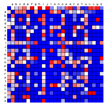
Figure 2: relative character pair frequency distribution for the sample
text, sorted alphabetically.
In this type of Figure, red colours indicate that certain combinations appear more frequently than 'by chance', while blue colours indicate that they appear less frequently.
It is of interest to look at some of the details in Figure 2. By looking at the row of coloured squares for "q", one sees that it is only red for the following character "u", as expected. Looking at the row for "x", one sees that this is preferentially followed by space, "i", "v", or "x". The combinations "xi", "xv" and "xx" are caused by Roman numerals that occur in the text.
The same Figures may be made by sorting the characters in order of decreasing frequency, which is shown below.
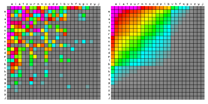
Figure 3: character pair frequency distribution for the sample text,
sorted by decreasing character frequency.
One conspicuous feature is the small square representing "space following space", in the upper left corner of both squares. In the left-hand figure it is grey, because this dooes not appear in the text. In the right-hand figure it is magenta (very high frequency). This feature will play a role in the following.
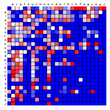
Figure 4: relative character pair frequency distribution for the sample
text, sorted by decreasing character frequency.
While the Figures showing relative frequencies (Figures 2 and 4) better highlight the character combinations that appear 'more than expected', they have the disadvantage that they over-emphasise some combinations that are still rare in the absolute sense. Both types of illustrations have been included here and here, and we will use both in the following.
![]()
The alternative procedure described above ("ALT" in the following) will now be applied to this text, for two states, while the space character is treated as a normal character, so may be assigned to either of the two states. This is the simplest possible scenario. The procedure starts with an a priori or initial 'guess', which is improved iteratively until convergence is reached. In the traditional approach, the a priori 'guess' is by assigning equal probability to all elements in the A and B matrices. Effectively, this means that all characters are equally likely to appear, which we already know not to be true. We will start by assigning equal probability to all states for each character in the R matrix. This means that the single character distribution is already taken into account (when converting R to B).
For this a priori case, the A matrix is the following:
  0.50000   0.50000


  0.50000   0.50000
and the vector of average state probabilities is the following:
0.50000 0.50000
We let the process run for 160 iterations. During each iteration, the simulated character pair frequencies are computed and compared with the actual frequencies. At the end of the process, all characters are distributed over the two states. This distribution is also probabilistic, i.e. a character may be emitted by both states with different probabilities. When looking at the result of the process, we assign each character to the state that is most likely to emit it. This turns out to be as follows:
State 1 ("vowels"):
space, e, i, a, u, o
State 2 ("consonants"):
t, s, r, m, n, c, d, p, l, b, v, h, f, q, g, x, z, y, j
The resulting A matrix is:
  0.28366   0.71634


  0.83211   0.16789
and the vector of average state probabilities is:
0.53738 0.46262
This result is quite positive, in the sense that vowels and consonants are clearly separated, while the space character is classified as a vowel. The solution score (the Bhattacharyya distance between the simulated and the true character pair distributions) is shown below, both for the a priori and final (converged) distances. These values do not mean much in an absolute sense, but can be compared for the different cases.
| Method | States | A priori | Final |
|---|---|---|---|
| ALT | 2 | 0.2176 | 0.1414 |
Using the Baum-Welch algorithm ("B/We" in the following), the first quantity we can compute is the nominal log(prob) value, which is: -3.6770 .
Also here, we will take the single-character distribution into account for the initial B matrix. After completion of the process (also 160 iterations), the following result was obtained:
State 1 ("vowels"):
space, e, i, a, u, o
State 2 ("consonants"):
t, s, r, m, n, c, d, p, l, b, v, h, f, q, g, x, z, y, j
This is identical with the result of the ALT method (10). The resulting A matrix is:
  0.20053   0.79947


  0.81365   0.18635
and the vector of average state probabilities is:
0.50440 0.49560
These are different from the ALT method, but it is hard to derive any conclusions from this difference. The solution score (the Bhattacharyya distance between the simulated and the true character pair distributions) is shown below, both for the a priori and final (converged) distances. In addition, the equivalent ('constrained') value for the ALT method (as explained above) is included. Finally, the final log(prob) value after convergence is shown.
| Method | States | A priori | Final | (ALT equiv) | Log(prob) |
|---|---|---|---|---|---|
| B/We | 2 | 0.2176 | 0.1389 | (0.1480) | -3.7497 |
This shows that the score for the B/We result is slightly better than for the ALT method, while its ALT-equivalent value is slightly worse. This is what would have been expected. The log(prob) value is a bit worse than the nominal value computed in advance.
Finally, as indicated before, we can compute the log(prob) value for the ALT algorithm by running one step of the B/We algorithm on its output. The resulting value is -3.7611. We may now collect the results in a single table, as shown below. Repeating values are not included.
| Method | States | Log(prob) | Score | (ALT equiv) |
|---|---|---|---|---|
| ALT | 2 | -3.7611 | 0.1414 | - |
| B/We | 2 | -3.7497 | 0.1389 | (0.1480) |
We may also plot the character pair frequencies again, where the characters have been grouped 'by state'. In these figures, the following conventions are followed:
The colour of the legend text indicates the different states, and they are also separated by yellow lines within the squares. As the two methods resulted in the same distribution of characters over states, the same figure is valid for both methods.
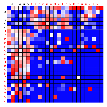
Figure 5: relative character pair frequency distribution for the sample
text, with the characters sorted by state (2-state HMM).
As described in the explanation above, the iterative procedure looks at the hypothetical character pair distribution of a simulated text. This simulated text is the result of running the HMM using the matrices that were estimated. We can also plot this hypothetical character pair distribution. This is also be done with the characters grouped by state, as in Figure 5 above. This clearly shows the effect of grouping all characters into two states, and reflects the fact that state-1 characters ("vowels") prefer to pair up with state-2 characters ("consonants") and vice versa.
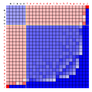
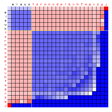
Figure 6: simulated relative character pair frequency distribution derived
from the sample text, with the characters sorted by state (2-state HMM).
Left: alternative method. Right: Baum-Welch.
These figures are almost exactly the same as the expected outcome of this process that was already illustrated in Figure 2 of the page discussing the HMM analyses. The behaviour of very low frequency characters can be ignored.
That both method were successful is clear from the separation of characters into what we know to be vowels and consonants. However, it will also be of interest to measure the success more quantitatively, using the two different score metrics, especially when we have in mind to apply the method to the Voynich MS text, of which we don't know if it can be separated into vowels and consonants.
The alternative method allows us to treat space characters as being emitted by a state of its own. We may call this a "2+1" HMM analysis, meaning that the third state is fixed to emitting space characters only, and the other two states will emit all non-space characters. For our source text, the probability that any character is a space (from counting) is 0.16758. To understand the a priori A matrix, it is best to look at the average state probabilities first. Non-space characters will appear at probability 1 - 0.16758, and these are split over two states. This means that the a priori average state probabilities are as follows:
0.41621 0.41621 0.16758
From this we can derive the a priori E matrix, knowing that spaces (state 3) never follow each other so the bottom right value is zero:
  0.16621   0.16621   0.08379


  0.16621   0.16621   0.08379


  0.08379   0.08379   0.00000
From this we obtain the a priori A matrix:
  0.39934   0.39934   0.20131


  0.39934   0.39934   0.20131


  0.50000   0.50000   0.00000
The result of the process is as follows, again after 160 iterations:
State 1 ("vowels"):
e, i, a, u, o
State 2 ("consonants"):
t, s, r, m, n, c, d, p, l, b, v, h, f, q, g, x, z, y, j
State 3:
space
This is essentially what we expected. The only change is that the space character moved into its own state. The resulting A matrix is:
  0.08949   0.74543   0.16507


  0.60183   0.16789   0.23028


  0.34785   0.65215   0.00000
and the vector of average state probabilities:
0.36980 0.46262 0.16758
Let us also run this scenario using the B/We algorithm, which in this case is still experimental. This appears to fail, and it is not useful to show the resulting distribution of characters over states. Instead, let us look at the statistics.
The a priori score is 0.1982 in both cases. This is better than the normal 2-state case, because the space character will no longer be allowed to follow itself. The other values have been added to the table:
| Method | States | Log(prob) | Score | (ALT equiv) |
|---|---|---|---|---|
| ALT | 2 | -3.7611 | 0.1414 | - |
| B/We | 2 | -3.7497 | 0.1389 | (0.1480) |
| ALT | 2 + space | -3.6922 | 0.1210 | - |
| B/We | 2 + space | -3.7832 | 0.1694 | (0.1902) |
The alternative method clearly has better statistics than for the normal 2-state case, also for the log(prob) value, which is now already close to the nominal value. It was computed by re-starting the B/We algorithm based on the output of the ALT method, and we also let this run for another 160 iterations to see if this allows it to converge better. However, this solution did not move away from its initial situation, so is not added to the table.
| Method | States | Log(prob) | Score | (ALT equiv) |
|---|---|---|---|---|
| ALT | 2 | -3.7611 | 0.1414 | - |
| B/We | 2 | -3.7497 | 0.1389 | (0.1480) |
| ALT | 2 + space | -3.6932 | 0.1214 | - |
| B/We | 2 + space | -3.7832 | 0.1694 | (0.1901) |
We will need to investigate the reason for this failure, or alternatively change the implementation such that it does not re-compute this state as a normal one.
The figure for the actual character pair frequencies will be identical to Figure 5, but let us look at the simulated character pair frequencies, to be compared with Figure 6:
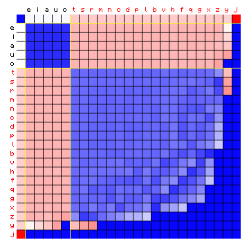
Figure 7: simulated relative character pair frequency distribution for the
sample text, with the characters sorted by state ("2 + 1" state HMM).
The fact that the space character does not behave like a normal text character, and this is modeled, improves the results.
For a three-state HMM, the B/We method is expected to deliver a reliable result, but the ALT method is still being tested. Its former implementation was known to be sub-optimal. The a priori A matrix is the following:
  0.33333   0.33333   0.33333


  0.33333   0.33333   0.33333


  0.33333   0.33333   0.33333
The result of the ALT processing is as follows:
State 1:
space, e, i, a, u, o
State 2:
t, m, d, p, b, v, h, f, q, g, z, j
State 3:
s, r, n, c, l, x, y
The vowels still include the space character, while the consonants have been split into two groups. The resulting A matrix is:
  0.28366   0.36789   0.34845


  0.92364   0.01956   0.05681


  0.72613   0.21305   0.06082
The result for the B/We processing is as follows:
State 1:
space, e, i, a, u, o
State 2:
t, c, d, p, b, v, h, f, q, g, z, y, j
State 3:
s, r, m, n, l, x
These results are similar but not the same. The space and vowels are again together in state 1. The consonants have been split over states 2 and 3, where the characters m, c and y are now in the other state when compared with the ALT result. The statistics have been added to the usual table:
| Method | States | Log(prob) | Score | (ALT equiv) |
|---|---|---|---|---|
| ALT | 2 | -3.7612 | 0.1417 | - |
| B/We | 2 | -3.7497 | 0.1389 | (0.1480) |
| ALT | 2 + space | -3.6932 | 0.1214 | - |
| ALT → B/We | 2 + space | -3.6906 | 0.1206 | (0.1219) |
| ALT | 3 | -3.7142 | 0.1331 | - |
| B/We | 3 | -3.6766 | 0.1285 | (0.1521) |
The problem observed already before, namely that the ALT result for 3 states is worse than the 2+space case, persists. This is a problem, because the 2+space solution was a possible outcome of the 3-state analysis, so a truly optimised solution should have been better. It would appear as if the same is true for the B/We algorithm, but here we need to keep in mind that this quantity was not being optimised. Instead, the optimised value 'log(prob)' has improved from the 2+space to the 3-state solution.
Some resulting figures are shown below. Figure 8 shows the simulated character pair statistics for the two solutions, now ordered by the character frequency, in order to be able to compare the two directly. While the yellow lines are not shown in this figure, the colour of the legend text (characters) reflects the resolved states.
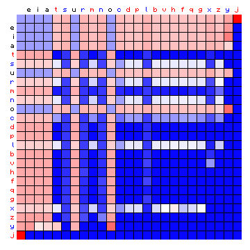
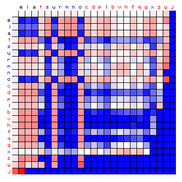
Figure 8: simulated relative character pair frequency distribution derived
from the sample text, with the characters sorted by frequency, for a 3-state HMM.
Left: alternative method. Right: Baum-Welch.
The a priori estimate for the 3-state case is identical with the 2-state case, as expected. An issue is that the 3-state HMM analysis could have converged on the same result as the 2-states plus 1 case. The score would have been better, but this did not happen. This is a convergence issue, that requires a close look, but may not be easy to resolve. In any case, the 3-state analysis provides an interesting result.
For this case, the "space state" is state 4, and the a priori average state probabilities are as follows:
0.27747 0.27747 0.27747 0.16758
The corresponding a priori A matrix is as follows:
  0.26623   0.26623   0.26623   0.20131


  0.26623   0.26623   0.26623   0.20131


  0.26623   0.26623   0.26623   0.20131


  0.33333   0.33333   0.33333   0.00000
The result of the ALT processing is as follows:
State 1:
e, i, a, u, o
State 2:
t, s, r, m, n, l, x
State 3:
c, d, p, b, v, h, f, q, g, z, y, j
State 4:
space
Again, the vowels have been kept together as a group, while the consonants have been split into two groups.
The B/We method, when applid to 3 + 1 states, appears to fail in much the same manner as before, and we may attempt the same remedy, which again turned out to be successful. The results have been added to the table:
| Method | States | Log(prob) | Score | (ALT equiv) |
|---|---|---|---|---|
| ALT | 2 | -3.7612 | 0.1417 | - |
| B/We | 2 | -3.7497 | 0.1389 | (0.1480) |
| ALT | 2+space | -3.6932 | 0.1214 | - |
| ALT → B/We | 2+space | -3.6906 | 0.1206 | (0.1219) |
| ALT | 3 | -3.7142 | 0.1331 | - |
| B/We | 3 | -3.6766 | 0.1285 | (0.1521) |
| ALT | 3+space | -3.5861 | 0.0977 | - |
| ALT → B/We | 3+space | -3.5001 | 0.0952 | (0.1135) |
The first thing to point out is that now, for both new solutions, the 'log(prob)' score is better than the nominal value (-3.6770). Also the matrix score has further improved.
The distribution of characters over states for the B/We method is shown side by side with the ALT method:
| State | ALT | B/We |
|---|---|---|
| 1 | e, i, a, u, o | e, i, a, u, o, x |
| 2 | t, s, r, m, n, l, x | t, s, r, m, n |
| 3 | c, d, p, b, v, h, f, q, g, z, y, j | c, d, p, l, b, v, h, f, q, g, z, y, j |
| 4 | space | space |
Only the two consonants l and x have been assigned to different states by the two algorithms. Of course, the two solutions cannot really be considered to be independent.
The ALT solution is shown below. Since the HMM algorithm minimises the difference between the absolute frequencies of the character pairs, it of interest to compare these directly, as well as the relative frequncies. In both cases the matrix on the left shows the original character pair frequencies sorted (and colour-code) by state, and the matrix on the right shows the case for the equivalent simulated text.
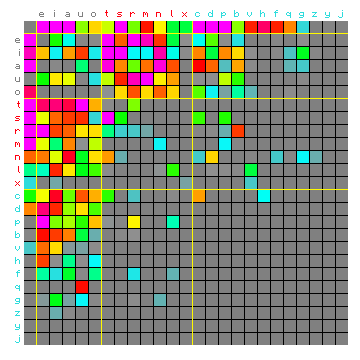
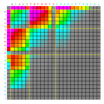
Figure 9: actual (left) and simulated (right) absolute character
pair frequency distribution.
The simulated matrix is based on the ALT method for 3 states plus a space-only
state, and the characters are sorted (and colour-coded) by state.
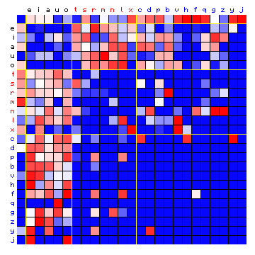
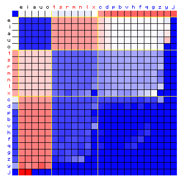
Figure 10: actual (left) and simulated (right) relative character
pair frequency distribution, for the same case as Figure 9.
In the Figures of the relative frequncies we can observe several larger blocks in the right-hand square, which are a reasonable average of the individual cells in the left-hand square.
It is clear that several important issues still exist, and these will be investigated:
On the positive side, the ALT method can now be run essentially for any number of states. The highest that has been attempted so far was a "9+1" state example which, while slow, converged to a realistic solution with a matrix score of 0.0551 .
The corresponding actual and simulated absolute frequencies are shown in Figure 11 below. This confirms at least in a qualitative sense that the 9+1 model was resolved successfully. Note that the left hand / first square only differs from the left hand / first square of Figure 9 in the ordering of the characters. The values for each character pair have not changed. In this case we see that the simulated case already begins to resemble the actual case. It is worth noting that the liquids "r", "n" and "l" have ended up in the same state.
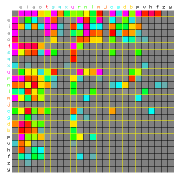
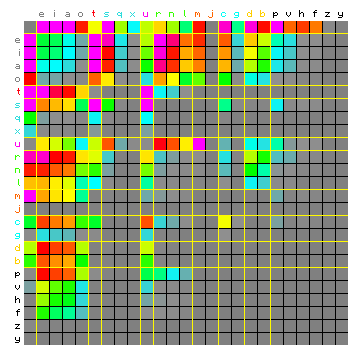
Figure 11: actual (left) and simulated (right) absolute character
pair frequency distribution.
The simulated matrix is based on the ALT method for 9 states plus a space-only
state, and the characters are sorted (and colour-coded) by state.
![]()
|
|
|
|
|