


|
|
|
|
|
There is the following famous phrase (which exists in several variations) (1):
If a monkey were hitting keys at random on a typewriter keyboard for an infinite amount of time, it will almost surely type any given text, including the complete works of William Shakespeare.
This provides a concept for "random text generation" that was already used by William Ralph Bennett in his pioneering analysis of the Voynich MS text using the computer (2). On this page we will follow in his footsteps. The material is quite straightforward, should be easy to follow, and may help to better understand some of the more complex material on other pages related to Voynich MS text analysis. It allows for some easy exercises and demonstrations.
In order to keep this simple, I will not be aiming for mathematically correct definitions, but more for descriptive ones.
In the following, I will use the word "arbitrary", and not "random", for processes that seem to happen without any method or according to any conscious decision.
As we will not be able to experiment with a live monkey typing on an actual computer keyboard, we will simulate this using a piece of software. Such software will need to include a "random number generator", i.e. the capability to provide us with an arbitrary number. Fortunately, such tools are generally available.
To keep it simple, we will use a keyboard that has 26 keys for the letters of the English alphabet, plus a space bar. Our piece of software could now arbitrarily select one after the other, each time with an equal probability of selecting any of the keys, independent of what the previous key was. The resulting text would be an arbitrary string, which would look nothing at all like a text in any language. Also, the 'apparent words' would be very long, because, on average, only one 27th of all characters is a space character.
If we now imagine that a human being were asked to stand in for the monkey, and arbitrarily type on the keyboard, he would not be able to be completely arbitrary. He would tend to follow certain patterns or preferences. For example, he might get into a habit of alternating his left and right hands, resulting in a preference of characters from the left half of the keyboard to be followed by characters from the right half, and vice versa.
Generally speaking, when we generate strings of characters based on some rules concerning which characters may follow each other, we are dealing with Markov chains, or Markov processes.
For the purpose of the present description, a Markov chain, or a Markov process, can be considered to be a process that generates a character based on the previous character or characters. If one searches for definitions on the internet (3), one will find more general (and more correct) definitions that tends to include the word "states", but for this simple introduction we can do without that.
For the case of the truly arbitrary (and hypothetical) monkey, the relationship between the most recent character and the following character is: "none". If this monkey has generated a string of characters, and we number these characters from the start (1, 2, 3, etc.), then at any position (n), the next character (at position n+1) is independent of the previous one. Also, the probability of all characters is the same.
In a real, meaningful text in any language, the situation is very different. Not all characters can follow each other, and the frequency of appearance of the various characters will be quite different. In English texts, for example, the space is more frequent than any character, and the most frequent non-space character will almost always be "e" (4).
In the following, when we talk about texts generated by monkeys or Markov processes, we will use a few rules to simplify things:
If we are interested in a Markov process that generates a text with the same character distribution as English, then we could start by taking an existing English text, and count how often each character occurs. If this text is 5000 characters long, and there are 850 space characters, then the frequency of the space character is 850/5000 or 0.17 . There could be 600 cases of an "e", so the frequency of "e" is 600/5000 or 0.12 , etc.
We could now define a Markov process that generates each character according to this character frequency distribution. However, each newly generated character would be independent of the previous one. The resulting text would still be nothing like English, but at least the frequency distribution of the characters in this monkey text would be the same as for English (assuming that we let the process run for a sufficiently long time).
The more interesting Markov chains are those, where the next character depends on the last character that was generated before. This matches the behaviour of real texts in English, where certain character pairs are reasonably frequent, others are rare, and some pairs are even forbidden. For example, "t" is often followed by "h", only rarely by "p", while "q" is never followed by "p". Throughout this page (and throughout this web site), such character pairs are called "bigrams".
If, for a Markov chain, the next character to be generated depends only on a single previous character, it is called a "first-order" Markov chain.
A very simple example of a first-order Markov chain is illustrated on the Wikipedia page (see note 3) (>>link to image ). We will use a similar case, but add a space character. This is done because the tools that I have set up for this type of text analysis all assume texts to be composed of words separated by (single) spaces. This modified example is shown in Figure 1 below.
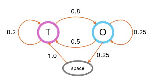
Figure 1: illustration of a Markov chain with transition probabilities.
This very simple Markov process can generate two different characters: "O" and "T" plus a space character. The transition probabilities are as follows:
In this simple case, all spaces are followed by a "T", meaning that all 'words' start with a T. Furthermore, the only character that can be followed by a space is "O", so all 'words' end with an "O". If we let the corresponding process run for a while, we will obtain a result similar to the following:
TOTOOTOO TTOTOTOTOTTTTO TOTOTOOTOTTOOOOOTOO TTOOTOTOOTTOOTOOOTOTO TOTOTTOTTOTO TO TOTOTOTOTTO TO TOO TOOTOOOTOTOTOTOTOTO TO TTOTOTO TOO TOOOTO TTOTTOTTOTO TO TOTOOOOTOTOTTO TOTOOTOTOOTO TTOTO TO TOO TTO TTOO TOOTOTTOTOO TOTOTOTTO TOTTOOO TOOOTOTOTO TO TO TO TOO TOOTOTOTOTOTOTOTOOTOTOTOTOOO TOTOOTOTOOOTOTOTTOOTOO TO TOTOOOO TOOTOOTO TO TTO TO TOTO TO TOTOTOTOTTOTTTOTTOOO TOTOO TOTTOO TOTOTOTOOTOO TO TO TOTTOTOOOTOOO TOOTO TO TOTOTOTOTTOTTOOTO TO TOTOTOTOOO TO TOO TOOTOTOOTOTOTTTOOTOOTOTOTO TOO TTOOTOTOTTOTOTOTO TOTOOTOOTOTOOTOTOO TOOO TTOO TOTOTOTOTOTOOTOTTOTO TTTOOOOTOTOTTTTOTO TTOTTOTTTOOTOOTOO TOTO TO TOTOTOTOTTTTOTTO TOOTTO TOTTOTOO TOTOTOTTOOTOTOOO TOTOTO TOOTOTTTTOTOTO TOO TO TOTOTTO TOTTOTOOTOTO
While this is not very exciting, we can observe a few things:
Let us now count the characters and character pairs (bigrams). The total number of characters in the above example (including one trailing space) is 711. Following are the single character statistics:
Table 1: single character counts and frequencies.
| char | count | frequency | expected |
|---|---|---|---|
| O | 334 | 0.4698 | 16/35 = 0.4571 |
| T | 301 | 0.4233 | 15/35 = 0.4286 |
| spc | 76 | 0.1069 | 4/35 = 0.1143 |
The expected values can be computed from the transition probabilities. We do not need to go into the details of how that is done (5). Let us just note that the statistics of the 'monkey' text are reasonably close to these expected values.
For the bigram counts, with 711 characters it would appear as if we had only 710 bigrams, but we can add the pair "space" followed by "first character", because there is an implicit space before the start of the text. Thus, we also have 711 pairs. Following are the counts, where the vertical direction gives the first character of each pair and the horizontal direction the second character:
Table 2: character pair (bigram) counts.
| O | T | spc | sum | |
|---|---|---|---|---|
| O | 91 | 167 | 76 | 334 |
| T | 243 | 58 | 0 | 301 |
| spc | 0 | 76 | 0 | 76 |
| sum | 334 | 301 | 76 | 711 |
Following are the frequencies, with those based on the counts on the left, and the expected frequencies, which essentially equals their probabilities, on the right. Again, the numbers are reasonably similar.
Table 3: observed bigram frequencies and bigram probabilities.
| O | T | spc | sum | O | T | spc | sum | |||
|---|---|---|---|---|---|---|---|---|---|---|
| O | 0.1280 | 0.2349 | 0.1069 | 0.4698 | O | 0.1143 | 0.2286 | 0.1143 | 0.4571 | |
| T | 0.3418 | 0.0816 | 0.0000 | 0.4233 | T | 0.3429 | 0.0857 | 0.0000 | 0.4286 | |
| spc | 0.0000 | 0.1069 | 0.0000 | 0.1069 | spc | 0.0000 | 0.1143 | 0.0000 | 0.1143 | |
| sum | 0.4698 | 0.4233 | 0.1069 | 1.0000 | sum | 0.4571 | 0.4286 | 0.1143 | 1.0000 |
In the above, we encountered probability distributions, where the sum of all probabilities is 1. The simplest example is that of the frequencies of single characters in a text. Such a set of numbers that add up to 1 are called a partition. I personally find it most convenient to think of this as cutting a cake into several pieces. The resulting pieces are the partition, where the sum, the whole cake, is 1. In this situation we are dealing with fractions rather than probabilities, but this is fully in line with the sense of characters making up a text. A character that appears with a frequency p (where p is between 0 and 1) has a probability of appearing at any point equal to p, and will take up the fraction p of the entire text.
People cutting a cake usually aim at creating pieces of equal size. A measure for the success in doing this is called the entropy of that partition. A high entropy means that all fractions in the partition are of equal size. A low entropy means that there are parts of very different sizes.
Figure 2: a low-entropy cake cut
As we know that the characters making up a meaningful text in any language will include a whole range of frequencies from (relatively) large to very small, the entropy of their partition will be clearly lower than the maximum.
We will not deal with entropy in the remainder of this page, nor with mathematics, so I will not include the formula here. This topic is elaborated further here (introduction) and here (first analyses). Even more details may be found here.
It may be useful to briefly explain how we can use a "random number generator" to select one item out of a partition. Going back to our cake, that has been cut into pieces of different sizes, if we were to throw a cherry on it from a distance, it will arbitrarily land on one of the pieces, but the probability that it lands on any piece is proportional to the size of that piece.
Figure 3 below shows how we can effectively use a random number generator to pick an item in such a situation. It shows a partition of a rectangle into four coloured pieces, numbered 1 to 4. The total size of the rectangle is 1, and the fraction of each piece k equals pk.
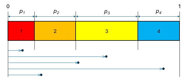
Figure 3: generating an arbitrary item from a list
Our random number generator now gives us a number between 0 and 1. Five examples of such random numbers are shown below the coloured rectangle. If this number is less than p1 , then we pick colour 1 (red). If not, we continue. Then, if the number is less than p1 + p2 , then we pick 2 (orange).
If not, we continue again, checking if our number is less than p1 + p2 + p3 etc.
In the above figure, the random number generator resulted in the sequence of colours: red, yellow, yellow, blue, orange.
Let us now go back to our case of bigram probabilities. The central square of the right-hand part of Table 3 is repeated below. This provides the probability of occurrence of each bigram:
Table 4: absolute bigram probabilities.
| O | T | spc | |
|---|---|---|---|
| O | 0.1143 | 0.2286 | 0.1143 |
| T | 0.3429 | 0.0857 | - |
| spc | - | 0.1143 | - |
The sum of all these numbers is 1. The way in which the first-order Markov chain generates a new character is by looking at the last character, and deciding what can be the next character.
In principle, every new character can be any of "O", "T" and "space", with the overall probability distribution: 16/35, 15/35 and 4/35. However, depending on the last character, the probability distribution will be different from this. We (and the monkey) can derive the probabilities from Table 4. If the last character was a "T", then we need to look at the probabilities of the next characters, given that the previous one was a "T".
The probability of 'some event', given that we have 'some situation', is called the conditional probability.
The absolute probability of the bigrams starting with T are (from Table 4):
0.3429 for "TO"
0.0857 for "TT"
The conditional probabilty of "TO" occurring, given that we already have the "T", is 0.3429 / 0.4286 , and the conditional probability for "TT" is 0.0857 / 0.4286 . These values are 0.8 and 0.2 respectively. We can compute these values for all three rows in Table 4 and obtain the following table of conditional probabilities:
Table 5: conditional bigram probabilities.
| O | T | spc | |
|---|---|---|---|
| O | 0.25 | 0.50 | 0.25 |
| T | 0.80 | 0.20 | - |
| spc | - | 1.00 | - |
Here, the sum of the numbers in each row is 1, and we recognise the values in this Table: they are the same as in Figure 1.
Now that we understand the principle how we can generate a monkey text that takes into account the actual bigram probability distribution of a language, we can try this out for a real case. Since we usually do not have the bigram frequencies for 'a language', we approximate this by counting the bigrams in a piece of text written in that language. The longer the example text used for this, the more realistic it will be.
We will do this for the sample text: "The fall of the house of Usher" by Edgar Allan Poe. We first make the text compatible with the criteria we listed near the beginning of this page, by removing all interpunction, converting any upper case characters to lower case, removing numbers and making sure that words are separated by exactly one space. Furthermore, a single space character is added after the last word. The resulting text has 40,094 characters. This text begins as follows:
during the whole of a dull dark and soundless day in the autumn of the year when the clouds hung oppressively low in the heavens i had been passing alone on horseback through a singularly dreary tract of country and at length found myself as the shades of the evening drew on within view of the melancholy house of usher i know not how it was but with the first glimpse of the building a sense of insufferable gloom pervaded my spirit i say insufferable for the feeling was unrelieved by any of that half pleasureable because poetic sentiment with which the mind usually receives even the sternest natural images of the desolate or terrible i looked upon the scene before me upon the mere house and the simple landscape
We cannot now tabulate all single character and bigram frequencies, but we can show the bigram frequencies in graphical form, for which see Figure 4 below. The first character of each bigram is along the vertical scale and the second is horizontal. So, for example, the bigram "th" is found on the row that has a "t" on the left hand side, and then searching horizontally to the column that has an "h" written over it. This cell is magenta. The corresponding cell for "ht" is light blue/cyan. Grey cells represent very-low frequency bigrams, and the frequency increases through cyan, green, yellow red to magenta. The leftmost column and the top row represent the space character.
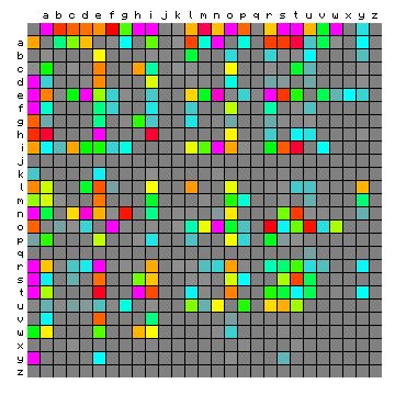
Figure 4: bigram frequencies of "The fall of the house of
Usher".
We can now let our first-order Markov chain run and generate monkey text. This starts as follows:
the iteadrvee therettof thinf ithithalecircaive ugondis ip mbofubesknervast uf of ammen whit d s ase jand ilurthuly tesa acart then a ha imay fat tomss te fe ade ilemisegs a tzedoorighe atis are ili mph ithe thereited h ons prvi d bry hagas iterellang he loated be thort thoflli klioro wime porand t f werd wanhead h assiman tede iof f aly arn the fun iseds nous youshind an whe sawichangerunindmed te ad wanteiealie mare t are het t scto wisewi t cemy t ond es ashe s issof t revoulerinter pof bhanthend nound orve cexallifopof t the w me atece ls w sougulenatrit antus genesheysthin wirtopowngape ond l waitidi osusi ttyernorat irpe inuthind astapers llllled anect ceanthitus piof ome ch wheatof inititharove mi earomofoneprs on and stan h ble ist mamppond whatindof pemenduthre frang e wadand ce f cralf inthiref wa ser se ed ure onsund led ar i
While this does not look like English, we do recognise some valid character combinations and even word fragments, and there are only very few character sequences that are completely unpronounceable.
Having let this run for 6000 characters, we can also compute the bigram frequencies of this monkey text. It is show below, side by side with the figure for the original text. These can be observed to be very similar, so the Markov chain was clearly functioning properly.
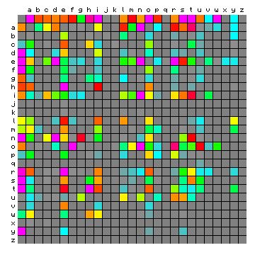
Figure 5: bigram frequencies of the simulated text (left) and
the original text (right - same as Figure 4).
We can now take this one step further. Instead of only looking at the last single character, to decide what should be the next one, we can also take into account the last two characters. To do this, we should know the frequency distribution of all groups of three characters (or: tri-grams) used in the chosen language.
While it is a bit more work, and appears a bit more complicated, the process is exactly the same as for the first-order Markov chain based on bigrams:
The initialisation starts with a first implicit space character, and the first real character can be chosen arbitrarily from those that can follow a space. After that, the process can run as long as we want, always looking at the last two characters and selecting a new character according to the trigram frequencies. This was again done for the same source text, and the result begins as follows:
pplant i wore themervid the of upowed gloul dwees thers in of it exprest to und de hill whis der apper mighaterew whick a dattered bable im whing tinso uplarcall ifells ouge sylly re pon the and ifeartaintembleas or of anded truch any feclon the of so gleas the bed itiquity spichaross withe of of the whient mor bin ang harat in in fe agul of the ful ing welts futrunted ancy felittemed low thered thad at nome he ene quen and few the vicusking thally tand i th the rallought pestreasint tarm cambeyed ingetand succe wasin the much havend as i aniguallonved frots ants hand upowy ing usittentrier he i have us theiver tousiroulon tim ints the ant of teming fle indid he viorus of careal lay ress amentmor
This looks like an eerie combination of garbled words, with some real English words thrown in, but an overall complete lack of sense (6).
While it may seem tempting to also try out even higher-order Markov chains, and obtain even more realistic-looking arbitrary text, this would only be possible if we had realistic quad-gram statistics for the language. (Quad-grams are groups of four consecutive characters). To compute these, one would need a very long sample text, much longer than the example used above. If we do this based on a text that is too short, then all low-frequency combinations will just become zero or one (out of N) and our random text will just start to repeat longer sequences from the source text. We will therefore stop at this point. A few more examples of second order monkey texts are given in Annex A below.
Let us go back to our first-order Markov chain above. As we know, this process takes the last character of the previous text, and generates one new character based on the bigram transition probabilities. Let us now consider that we don't work with all different characters at each step, but just with groups of characters. We may use three groups, which we number 1, 2 and 3. At every step of the Markov process, our monkey takes the most recent group (1-3), and generates a new group (1-3) based on the bigram frequencies between these groups. Now this does not give us a text, but just a string of numbers 1-3. To convert this string into a text, we can use a second monkey.
So let us imagine a monkey with a typewriter with just three keys (1-3) and whenever he hits a key, a lamp will briefly light up above one of three keyboards of a second monkey. We may call this first monkey the hidden monkey, and we see only the second one. This second monkey has been trained to hit a random key on a keyboard, whenever the lamp above that keyboard lights up. Each keyboard has different sets of keys, representing one group of characters.
One example of this subdvision into groups is: group 1 has all vowels, group 2 has all consonants and group 3 just has the space character. In order for this process to generate something that looks like real language, the rules for the first monkey must be based on the frequencies of vowel-consonant-space pairs, and the second monkey should generate the characters in each group depending on their relative frequency. This combination of two different processes is called a hidden Markov chain (or process).
The interest of hidden Markov processes is, that there are methods that take an existing text, and can estimate the combination of groups that best approximates this text. These methods are referred to as "Hidden Markov Modelling" (HMM). In literature about hidden Markov models, the groups are always referred to as 'states'. The user only has to select how many groups (states) he wants to use. These methods are the topic of this page.
Without repeating the details here, the properties of the 'hidden monkey' in this process are defined by the matrix A described on that page. The matrix in Table 5 above is an example of such an A matrix, while Table 4 represents an E matrix, as discussed on the same page. The combined properties of the 'visible monkey' are containted in the B matrix.
Following is a short example, which should be understandable even without knowing the details of how these algorithms work. We apply a 4-state hidden Markov model to our source text: "The Fall of the House of Usher", which will split the text into four groups, where one of these four is pre-defined to include only the space character (7). Following is the resulte:
Group 1:
e, a, i, o, u
Group 2:
t, h, c, m, w, p, b, v, q, j, z
Group 3:
n, r, s, d, l, f, g, y, k, x
Group 4:
(space)
We see that the vowels are all together in one group, while the consonants (including "y") are split over two groups.
We may now also let this hidden Markov process run and let our duo of monkeys generate some arbitrary text. This looks as follows:
dtbab tslg es hul arleve rf macue s o nitarn gedesaaths n n eemosnenan an pn enenhifs eza cinoferasara thos her w en heda rsatahtrnefbbogosasd lhidas a ryadtatwhapatmete it tunwa wfy s habemuntil spaonevi taname ine n fu vtnak irt orial wiy adgoineny hlgliyeh in topabanorefuofyhh beg edgs s ul c hecahun oik o l n wnay sto tfadsatiferg y htiret hler grl atafmos nsesd tehef todrun h cidv se meuthehen ahuf h oliramrif heriaipo in crid g ota tolidien yista ibuwen o dd t eu lir pibanb ca hiertenid i hi l o t ef w nat ir uotp hahhalo os meh lcihcad hf e hyefod peh bo ele r pesrtk hetlsaadtiddor wighoso tybateshas oleushi ol er r tesm e trcont e i ddihdahu o osl heye idoddnamtd nneikn s co hu eee ara
This looks nothing like English, and the corresponding bigram frequency graphic may help in understanding why: the frequencies of bigrams have to some extent been 'smeared out' over the characters within the same group. This is shown below in Figure 6, with the monkey text on the left, and the original text on the right.
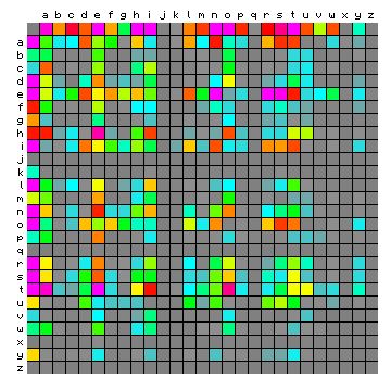
Figure 6: bigram frequencies of "The fall of the house of
Usher". Hidden Markov text left, original text right.
This becomes even more clear when we redo these graphics with the characters sorted by their groups (Figure 7 below).
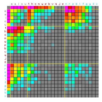
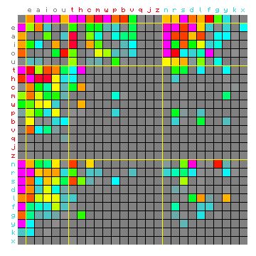
Figure 7: bigram frequencies of "The fall of the house of
Usher". Hidden Markov text left, original text right. Same data as Figure 6,
only sorted differently.
Just because of its entertainment value, here are some additional texts generated by first and second order Markov chains (a.k.a. monkeys). The three Latin texts are of very different origin, which appears to be reflected in subtle differences in the flavours of the monkey texts.
Starting with a first-order monkey text:
rno itae tumabunisetus eritinimumiundedeprc dulgues itulir idiex duosesu quat bo d gnerauntuacera realali hetitexcuntate a ant quns a fe hecuramo ss ss s dera cocefflitent a quimquridio atora olem i is aetem qumnentam e m s orus de purce gocet s mbeno elalo s ia edolunt sit qum isdior vilidiondenis emumociuglmelalia qunecibulir gndec advi nt repadum isenulisttaxussesaecam tederext iciontumineten que caugnuincelicenaquit aniaecudpaquss vorexs s cervit maem t arie pagrqucis plutuiloniuis nnddae iurcollistenintui cex eridono is selat im ataea is varmo vemidusiua lutodeminthivuscte ttostinusiinccnim i uletqus nturi suusprro s hora inusctem arugnctualllliem alilubegintistus nio ciiidam viquss aemitruocorui io derrerctenttudinc inort m e cim ist
And a second-order monkey text:
rti is faut latortiusa et soliis que esalic exces simus in lapiudatroitu ruit alia foniatotu est ariac me gessolydo serga bast que c ae ae exoris statumin et actem florint a rum tis et derri ano ine ina hum diemines in alit oruna ignundeffices similique con simaccatitit soperofactions vigientibus quagrargium porae c rhoens signalibra adve no sim exiidines lusa volstread maximarius inem pulstatin qua cauratereaec in ples ant est scontravis vi se eturnantem ta que partur in potus gregyptant cae itrannonsum inove ceu fonctordit sidat in atii allauctus ventestiulantur et muntutresnestituravirculgone idulevoctantura suuntisces gno afruras il prahertam nondeferies cilius sur nis cone co vis st ae prosperribent deorenitantro med ingus maia in int
Again, the second-order text is far more 'interesting' and in the following we will not generate any more first-order texts.
ute hujudiver temantus et sigististia esto aet fratemorips menit et tervant ta magis grautes est aut idem haediculum et calent quid abebapiet est sum serae ne dicarem sicui aut ipsorem ejus catia es loc evanctimod virifacescitus es qui enim gratent mi es judiced gloquis sit qui inequi voc confidem alium esuideni jes qui es sedi hoc cad vobis sigante homit mus exspirobil entem pete imensiverecum bobibeat num esseccedicat con esuaratest vos vobibentus arim et con audet quis potus homis quid eni lus perestinctut ad ventemone in si do mea sed ant vansi verietist corungeliquidus jundum tristur ne min has et et novir suuntisi santia hostis il ipirest infiens anibulienstorute non dei ens vos suaecersus et uncri estrem sicituloquaecrit ne addaecut
lpia sem vulontritosto diestis virtum et pe dum unum sue nananat dolortuambat coli et pestos dei alia ad biosonet teratia capulvere acci et vidim ut subio et capilibermist abitemplas is ason alia et is adier si quis her maremixi cocutem dei et siciper fem ratium et itorcum cum adierendum inegnandum eto serum qua gid supe ino is folia bitum quist dolentius heriguterbeni bibus et vice is pulvento alia emplaut de in mam et cribe sanascur virmum sam ovis herbata nia iderit is istrum spatiude es essuperbentur istre deu cum spatium macta es sem adicuisto ventius vel tur et osicuto si trostius indo poredatifiret proptatutius nas fore flus que alum dis herem in medice et prost pla de es handum salictontum subito dectam sibus come firtum de de et sanam
nto er iiii l soltorto cononciato via e mi a vedi si ste parbelta tro quanza che d e gratorta ebbasper la giudi verciasi a cli quesi accacchiegno spero se di a per grestir a qualtrodalo buosa oh e l lo aette perne te il mendonto ch isse dio er si mai accagnati che simmo soscon alto mi vide non la quaio quesolsi che anto di se parla e chio mi si a vi gra ventro voltore da do del voce le puore si anda davaiu ne fia l pero ali desie pero vollor sa e vol mi fata pie paronfentemmoste pinten pied e lun percire inose chi dicere discon co in aper altesappreva perreta lutte li trizzo personto lusse deli ch un tu santroccostroltrar lieggiostigli amo l su mile e da mer che trostrai pagil che vinassa giustro misi in dinseghia poscia bentor macceni fura
n hete onso merenincsen ghi hi bidde achte ens al willeest sit bedatterm moecande en op u vre daenen sede onsekel u wilde ninc wast eet en dlande voors vie conin oninde hoe enbeslort hi nu ve lie te scaeswas gode hooreen slastroen icken die of gode so si so vin inen varecht man sconthebren coninene dic vingerde is denen dier op daen eenre coer hent eninem scht ystadde de doet hijt sint moerende en de ic hoet die te mi we coniewel mijt brooft gen huut steende ghe menden scamerwan mangel lie is hover hielen hagheens alderen scilde u hi el onender mac feliemach endie diendenghi waertels clucel dat dievende westuch mouwerte wen wi sakende iete hewren conin iseit inendendie conien onin bidest en mocht hal en en lant wastal hi en hin hen die sch
NOTE: the following section describes the verification of the software implementation of the two algorithms described on this page. This part will be of little interest to most readers.
With the monkey processes described on the present page, it is possible to generate a text that would be an exact result of a hidden Markov chain. This text can then be used to verify the proper functioning of the above-mentioned software implementation.
For this, we set up a hidden Markov process along the following lines: three groups of characters and one group that includes only the space character:
We allow the following combinations:
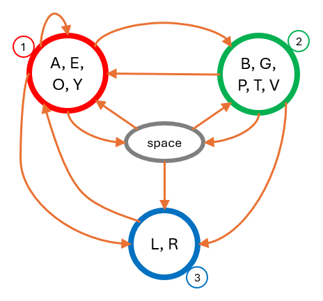
Figure 8: state and transition diagram for the simulated text.
The selected state transitions are given below, first showing the conditional state transition probabilities (A matrix):
  0.075   0.500   0.200   0.225


  0.400   0.000   0.200   0.400


  1.000   0.000   0.000   0.000


  0.300   0.450   0.250   0.000
From this follows the vector of average state probabilties (P vector):
0.366603 0.268805 0.174584 0.190008
... and the matrix of unconditional state transition probabilities (E matrix):
  0.027495   0.183302   0.073321   0.082486


  0.107522   0.000000   0.053761   0.107522


  0.174584   0.000000   0.000000   0.000000


  0.057002   0.085504   0.047502   0.000000
The selected B matrix, giving the distribution of characters emitted by each state, is shown below (where the underscore represents the space character):
--  --1--   --2--   --3--   --4--


_:  0.000   0.000   0.000   1.000


A:  0.200   0.000   0.000   0.000


E:  0.400   0.000   0.000   0.000


O:  0.200   0.000   0.000   0.000


Y:  0.200   0.000   0.000   0.000


B:  0.000   0.100   0.000   0.000


G:  0.000   0.200   0.000   0.000


P:  0.000   0.300   0.000   0.000


T:  0.000   0.300   0.000   0.000


V:  0.000   0.100   0.000   0.000


L:  0.000   0.000   0.400   0.000


R:  0.000   0.000   0.600   0.000
The monkey text can be generated in two ways, either by running a hidden Markov monkey, or by computing the expected bigram frequencies and use these as input for a normal first-order Markov process. We aim for a text of 24,000 characters. As the monkey generates complete words, it ended up with 24,015 chracters. The second option turns out to produce a text that is closer to the expected frequencies, so this will be used here. The character frequencies are shown in the following Table, with the expected frequencies on the left, and the actual ones of the monkey text on the right.
Table 6: single character frequencies of the monkey text: expected (left) and actual (right).
| char | expected | actual |
|---|---|---|
| (spc) | 0.190008 | 0.18813 |
| A | 0.073321 | 0.07312 |
| E | 0.146641 | 0.14749 |
| O | 0.073321 | 0.07391 |
| Y | 0.073321 | 0.07466 |
| B | 0.026881 | 0.02507 |
| G | 0.053761 | 0.05305 |
| P | 0.080642 | 0.07908 |
| T | 0.080642 | 0.08249 |
| V | 0.026881 | 0.02723 |
| L | 0.069833 | 0.06758 |
| R | 0.104750 | 0.10818 |
We can observe that the frequencies are reasonably close, but not very close to the expected values, and we would need a clearly longer text in order to do better, but the text length is a major factor for the traditional Baum-Welch algorithm, so we will work with this example.
The algorithm needed over 350 iterations to reach a stable solution, and all characters were assigned correctly to their states. The algorithm numbered the states differently, and in the following they will be renumbered to match the example of Figure 8. The resulting average state probability vector P is given below, and compared with the expected one:
Table 7: Average state probabilities from Baum-Welch (left) and expected (right).
| State | computed | expected |
|---|---|---|
| 1 | 0.3664 | 0.366603 |
| 2 | 0.2689 | 0.268805 |
| 3 | 0.1757 | 0.174584 |
| 4 | 0.1889 | 0.190008 |
The detailed distribution of characters over states is given by the R matrix, which should ideally have values 1 for the matching state and 0 for all other states. The result is shown below, with the states renumbered as in the example above:
--  ---1---   ---2---   ---3---   ---4---


_:  0.00000   0.00000   0.00000   1.00000


A:  0.98594   0.01406   0.00000   0.00000


E:  0.99502   0.00000   0.00000   0.00498


O:  1.00000   0.00000   0.00000   0.00000


Y:  0.98689   0.01304   0.00000   0.00000


B:  0.00000   1.00000   0.00000   0.00000


B:  0.00000   1.00000   0.00000   0.00000


B:  0.00000   1.00000   0.00000   0.00000


B:  0.00000   1.00000   0.00000   0.00000


B:  0.00000   1.00000   0.00000   0.00000


L:  0.00000   0.00000   1.00000   0.00000


R:  0.00000   0.00000   1.00000   0.00000
This is a nearly perfect result, apart from very minor deviations of 1.5% or less for the vowels (state 1). This is presumed to be caused by the fraction of vowels that are allowed to follow each other, where the actual frequencies in the text are not perfectly aligned with the expectation.
In general, we may consider that the implementation of this algorithm is correct (8).
In this case, a space-only state is pre-defined, and only three additional states are estimated. We may call this a "3 + 1"-state solution. This method required approximately 30 iterations to reach a stable solution, but that is certainly optimistic, and due to the fact that an exact solution exists for this problem. Also in this case, all characters were assigned correctly to their states, apart from the different numbering. The resulting average state probability vector P is given below, and compared with the expected one:
Table 8: Average state probabilities from the alternative method (left) and expected (right).
| State | computed | expected |
|---|---|---|
| 1 | 0.3692 | 0.366603 |
| 2 | 0.2669 | 0.268805 |
| 3 | 0.1758 | 0.174584 |
| 4 | 0.1881 | 0.190008 |
While in this case, the state probabilities differ a bit more from the expected values, they match exactly with the actual character probabilities of the input text. Following is the R matrix, which exactly matches the expected one.
--  ---1---   ---2---   ---3---   ---4---


_:  0.00000   0.00000   0.00000   1.00000


A:  1.00000   0.00000   0.00000   0.00000


E:  1.00000   0.00000   0.00000   0.00000


O:  1.00000   0.00000   0.00000   0.00000


Y:  1.00000   0.00000   0.00000   0.00000


B:  0.00000   1.00000   0.00000   0.00000


B:  0.00000   1.00000   0.00000   0.00000


B:  0.00000   1.00000   0.00000   0.00000


B:  0.00000   1.00000   0.00000   0.00000


B:  0.00000   1.00000   0.00000   0.00000


L:  0.00000   0.00000   1.00000   0.00000


R:  0.00000   0.00000   1.00000   0.00000
In this case, all four states were estimated without any further assumptions. Also this method required approximately 30 iterations to reach a stable solution, which is again optimistic for the same reason.
The result can be described very easily, as it is completely identical to the "3 + 1"-states solution.
Both the Baum-Welch implementation and the alternative implementation have been verified to work properly.
![]()
|
|
|
|
|